SIMarchitect Tutorial

This Tutorial elaborates and demonstrates the interface of SIMarchitect and functions as a step-to-step guide for creating a simple model. This section is intended for first time users. A fully worked-out example is found in SIMarchitect. From Start-Up, select Open Example. If the work-out example is used, jump to Adapting Model The other option is to build the example using the guide below.

The complete Example Model can be downloaded here. This model can be used for comparison and troubleshooting.

Creating a model

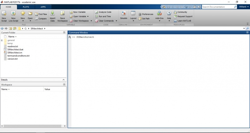
To create a new model in SIMarchitect, the first step is to open MATLAB®. Navigate to the path in which the SIMarchitect.m file is located (root of SIMarchitect) and in the Command Window, type SIMarchitect and press enter (Command is case-sensitive). An initialisation occurs: Initialisation of SIMarchitect successfull Please type 'SIMarchitect' to start. Here, type SIMarchitect and press enter to start the programme. After first-time use, it is necessary to enter the command only once.

Now SIMarchitect will load libraries and directories. A prompt will appear at every new startup of SIMarchitect asking to save a new path. Click 'Yes'

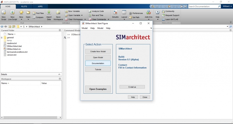
Next, the SIMarchitect Start Figure appears. Click on 'Create New Model' and save the model to the desired location.

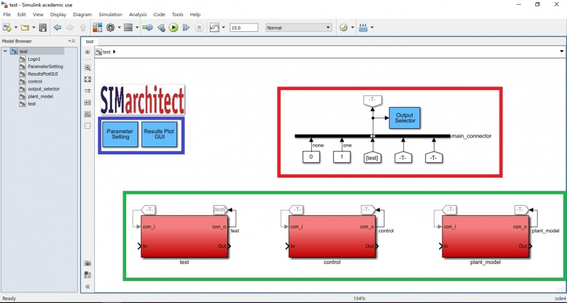
A new model in the SIMarchitect environment is opened. A SIMarchitect model has several unique features. Starting with the 'Component Blocks', which are inside the green area. These three blocks are part of every SIMarchitect model:

• Test: This is where the test protocol is modelled. All variables and parameters related to testing the system are to be placed here.
• Control: The control system is to be placed here. The control system controls the response between the test input and the plant model response.
• Plant Model: The plant model is the model of the system which is simulated.

Next, the components inside the red area. This is the main connector. The main connector is the point where all signals of the model are merged into one data bus, which can be used to analyse results. The desired signals can be selected in the 'Output Selector' by double-clicking on this block. The signals selected here are saved to the data bus and MATLAB® workspace for analysis.

Finally, the components inside the blue area. These components are the 'Parameter Settings' and the 'Results Plot GUI'. The parameter settings are a way to define parameters of each sub-component. The results plot GUI is a fast way to plot results for analysis.

Building a simple model

The next step to modelling in SIMarchitect is to build a simple module.

For this tutorial, let's model a simple equation: y = a * x + b with:

• a = 2
• b = 5

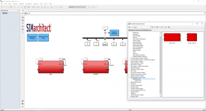
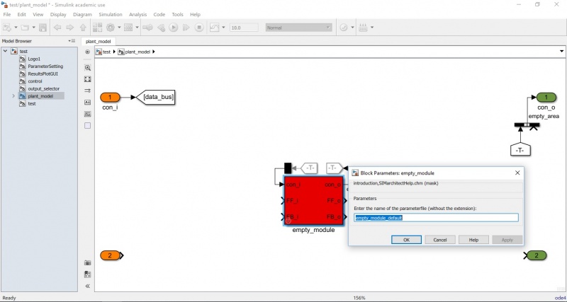
All modelling in this example will be done in the 'plant_model' component. The plant model component contains all modules related to the plant model. In this case, the equation is the plant model. First, add an empty_module from the SIMarchitect Library. This difference between and empty_module and empty_component is that the first can be assigned a parameter file and the latter cannot.

Double click on the module to type the name of the related parameter file.

Next, type the parameter file name 'experiment'. This ensures that the empty_module searches for an .m file called 'experiment'. As this file has not yet been created, we will do that now.

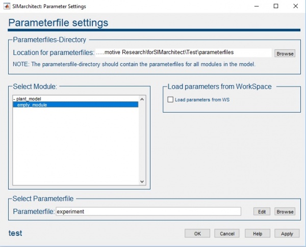
Navigate to the top-layer of the simulation model and double-click on the 'Parameter Setting' subsystem. This opens the window seen below. First, check the 'Location for Parameter files'. This is were the model searches for the parameter files. This should be in the location where the example model was created, inside a folder called 'parameter files'. Now, we will assign the parameter file to the component. Expand the plant_model tree under 'Select Module' and select 'empty_module'. Then, under the 'Select Parameter file' heading, click 'Browse'. This opens a window in the specified location. This window contains the file 'empty_module_default.m', which is placed by default when a new empty_module is added to a model. Rename this file to 'experiment.m' and click open. Now the parameter file selected is 'experiment'.

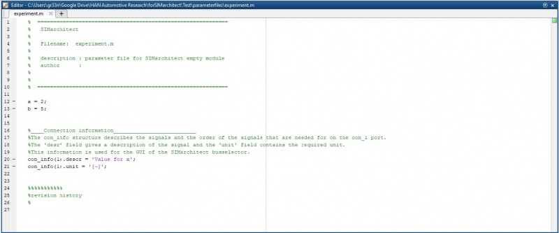
In the parameter files window, click 'Edit'. This opens the .m file in which all the parameters are stored for this example. There are no parameters defined yet, so that is the next step. Delete the unnecessary information in the file, to keep a clear overview. Also, in the commented section, fill in the filename 'experiment.m'.

Fill in all of the necessary parameter of the module inside the parameter file, together with the connection information. For this tutorial, a and b are the parameters so these must be defined inside the parameter file. Use a = 2 and b = 5. Then, in the 'Connection Information' fill in the values seen in the figure.

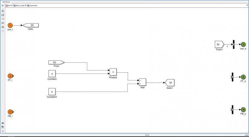
Next, create the simulation model. Navigate to the plant_model and rename the empty_module to 'experiment'. Then open the 'experiment' component. To do this, click on the small arrow located on the lower left of the module block. The text in the centre of the model is a description on building in SIMarchitect. This can be deleted when read.

There are two sides of the module which represent the input port and the output port:

• Left side (orange ports): All of the input signals to the module
• Right side (Green ports): All of the output signals from the module

Important to know: In SIMarchitect styling, signals between input->model, and model->output are connected with 'go-to' and 'from' blocks instead of lines. This is shown in the figure below. Build the model as seen in the figure, and name the output signal (to 'con_o') appropriately. In this case, the signal line to the output port is named 'y', and this is how it will be described throughout the whole model.

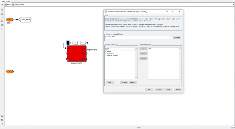
Finally, connect the input signal to the module by selecting the appropriate signal in the bus selector prompt. Do this by navigating up one level, and double-clicking the black rectangle on the input port of the experiment module. This opens the bus selector window. For this step, we will use 'one' as an input, but signals from the whole model can be entered to use as an input.

All of the signals available in the simulation, which are connected to the main bus connector, are displayed in the signal in the bus box and connect the signal according to the order of the connection inside the module if the module requires more than one inputs.

Plotting simulation result

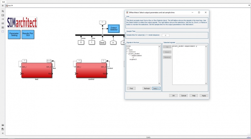
Navigate to the top-layer of the simulation model. Double-click the 'Output Selector' block to select which signals are going to be displayed in the 'Results Plot GUI' function.

For this tutorial, choose plant_model -> experiment -> y. This is the output of the plant_model.

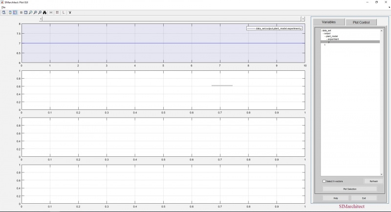
The result simulation can be viewed by using the 'Results Plot GUI' function.

All selected signals are seen in the right-hand panel. Double-click to plot the signals in the selected graph.

To view more signals, connect more parts of the plant_model to 'goto' and 'from' blocks, and connect these blocks to the bus (output of plant_model). Name these signals and select in the output selector. These signals are also sent to workspace with the name 'data_set' and in a structure data-type.

Adapting Model

In this section, the Example Model will be adapted and extended. If the first part of the Tutorial has not been done (using the pre-built SIMarchitect model, make sure the parameterfile of the eq1 module is correct and the inputs to eq1 are correct (see above).

First, we will add a new module. In this module we will create a second equation.

1. Add a new empty_module (From SIMarchitect General Library) to the plant_model, and name this 'eq2'.

2. Now we will build the equation inside the 'eq2' module. The equation to build will be: y2 = a2*x2^2 + b2*x2 + c2*x1, where x2 is an increasing value and x1 is the output of eq1.

3. Build the eq2 module to match the system seen below. The parameters a2, b2, and c2 will be defined in the parameterfile of this module. The Ramp block has the following parameters:

• Slope: s
• Start time: t_start
• Initial output: init

These values will, also, be defined in the parameterfile.

4. Add any signals to the output that you wish to monitor. For this example, y2, x2, and x2_sq are chosen, but others may be added. Remember to name the signals heading into the output bus, or these will not be discriminable in the rest of the model.

5. Now, create a parameterfile for this block. Double-click on the eq2 module and change the name of the parameterfile to eq2. Then, in the top-layer of the model, select Parameter Settings -> expand plant_model -> select eq2 -> click Browse (bottom-right corner) -> this opens the browser to select parameterfiles. Rename the 'empty_module_default.m' to 'eq2.m' -> Select the file -> open. In the Parameterfile settings window, click apply (don't close the Parameterfile settings window yet).

6. Now the parameterfile has been assigned, we can enter the parameters. Make sure 'eq2' is selected and click edit. This opens the parameterfile in Matlab. Enter the following parameters to the file.

• a2 = 6
• b2 = 22
• c2 = 2
• s = 1
• t_start = 0
• init = 0

Also, fill in the connector information:

• con_info(1).descr = 'x1';
• con_info(1).unit = '[-]';

The con_info(2) may be deleted as there is only one input to eq2. The parameterfile should be the same as the figure below.

7. Go back to the SIMarchitect model and close the Parameterfile settings window by clicking OK. Now we must match the correct inputs and select the desired outputs.

8. At the input port of the eq2 module, double-click on the bus selector (black box on input line). Remove the signal 'none' from the right side and add the plant_model -> eq1 -> y to the selected signals. Now the input signal to the eq2 module is the output of the eq1 module.

9. Next, on the top-layer of the model, open the Output Selector and select the desired outputs. In this case, plant_model -> eq1 and eq2 have been selected.

10. Now all the parameters are defined and all inputs and outputs have been selected, the model can be simulated. Simulate the model for 20 seconds, using a fixed-step solve (auto) with step-size 0.01s.

11. Open the Plot GUI and analyse the outputs of the simulation. Then, change the parameters for eq1 and eq2 and simulated again. Also, add more outputs to the data buses of individual modules to analyse more signals. Remember to always name the signals leading to the bus.

Assigning New Parameterfile

One of the useful features of SIMarchitect is the use of parameterfiles which are assigned to modules. This way, simulations for different parameter sets are easily run and analysed. For this section, the parameterfile for the eq2 module will be replaced with a different set of parameters.

1. Create a new parameterfile for eq2 by copying and pasting the eq2.m file. Rename this file 'eq2_set2.m'. Note: Copy-pasting the parameterfile can be done in the Matlab navigation panel, or in the standard file browser of the system.

2. Change the parameters of the file to the following:

• a2 = 45
• b2 = 5
• c2 = 22
• s = 2
• t_start = 2
• init = 1

Save the parameterfile.

3. In the SIMarchitect model, open the Parameter Setting and assign 'eq2_set2.m' to plant_model -> eq2. Do this by selecting plant_model -> eq2 -> Browse (right bottom) -> select parameterfile. Click apply and OK.

4. Open the plant_model of the SIMarchitect model and double-click the eq2 module. This opens the window for selecting the name of the parameterfile. It should have been changed to 'eq2_set2'. This indicates that the new parameterfile will be used. Note: It is also possible to type the name of the new parameterfile in this window, so it is not necessary to do this through parameterfile setting. Make sure the parameterfile is in the correct directory.

5. Simulate the model for 20 seconds, using a fixed-step solve (auto) with step-size 0.01s with the new parameterfile. Then, set the parameterfile of the eq2 module back to 'eq2', and simulate again.

6. In the Results Plot GUI, there will be a set called data_set and a set data_set1. The first set (data_set) is the newest simulation run result, in this case the original (eq2) parameters. The second set (data_set1) contains the results of the second parameter set (eq2_set2). Plot these results and compare the plots for both parameterfile settings. Example results can be seen below.

This figure shows the comparison of the simulation with two different parameter set inputs. The blue lines represent the first set (eq2 parameters) and the red lines the second set (eq2_set2).

Return to the main SIMarchitect page.