Autodock Model Tutorial

This page is a walk through of the simulation and 3D animation of the Autodocking procedure for a single-articulated vehicle. The page will explain the functionality of the Simulation model and its components, and the connection between the 3D animation model and the simulation results. The result of this walk through is a visually attractive animation in which the 3-dimensional objects (tractor and trailer) visualise the results of the simulation model. The goal of the simulation model is to have the vehicle (truck) follow the reference path, which is an input to the system.

Simulation Model

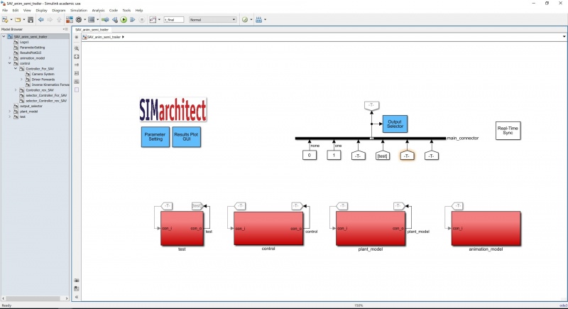
First, open the Simulink model (SAV_anim_semi_trailer.slx). The model will open at the top-layer. The top-layer of the model shows the four main components: Test, Control, Plant Model, and Animation model. The first three are part of the simulation model, and the fourth is the animation model. This can be seen below.

Test

Inside the test sub-component, several parameters are controlled that are specific to this situation. The vehicle follows a pre-defined reference path. Linked to this reference path are the starting point, the switching point from forwards to reverse control, the final location of the vehicle, and the initial conditions of the vehicle. For information about each of the components inside the test sub-component, descriptions have been added to the simulation model. (Double-click on the test block)

Control

Inside the control sub-component, the steering angle required to follow the reference path is calculated. There are two controllers: forwards control and reverse control. As these controllers are nearly exactly the same, only the forwards control will be elaborated. To open the sub-component 'Controller_For_SAV', click the arrow in the bottom-left corner.

Here, there are three areas:

• Semi_pos: This is where the steer-axle and the drive-axle are determined. For forwards are reverse, these are the inverse of each other. The steer-axle (the axle FINISH!!!!!!
• Driver Forwards: This is the driver of this model. The inputs are velocity of the trailer, the position of the trailer, and the heading of the trailer. These inputs are then used to calculate the steering angle (at the steer-axle) necessary to keep the rear-axle of the trailer on the reference path. So, the goal of the controller is to let the real-axle of the trailer follow the path.
  • Inside the Driver Forwards component (double-click on the grey area), there are two errors defined. The lateral error (distance from the vehicle to the path) and heading error (difference between the reference heading and the vehicle heading). The content of these error calculations will not be handled during this tutorial.
• Inverse Kinematics Forwards: The output from the controller is a steering angle for the rear-axle of the trailer. This axle, however, is not steerable. Therefore, the steering angle must be translated to the front axle of the tractor, which is steerable. The translation is done on the basis of kinematic equations. These equations will not be handled during this tutorial.

The first part of the simulation is in forwards control. Then, after t_for, the steering angle is taken from the reverse controller.

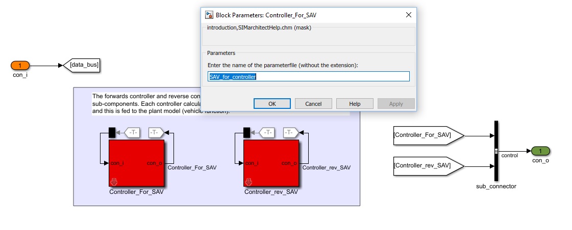
CHECK: Double-click on the Controller_For_SAV. A prompt opens (seen in figure below). Make sure this name of the parameterfile is: 'SAV_for_controller'.

Check this for the Controller_rev_SAV, also. Make sure this name is: 'SAV_rev_controller'.

Plant Model

The Plant Model sub-component, contains the vehicle function. The vehicle function simulates the tractor and trailer for this model. The inputs (tractor velocity and steering angle) are used to calculate the vehicle coordinates and states. Furthermore, some output values are re-used as input values. These values are the 'feed forward' values. The outputs are derivatives, which are looped into the input, integrated, and used to calculate the next iteration of the model. The kinematic equations will not be handled during this tutorial.

Animation Model

The final component is the sub-component of the animation model. This is where the simulation results are translated to values that can be used in the 3D animation. The 3D animation model uses a Virtual Reality world (VR Sink) in which the objects are driven by the results of the simulation model.

Signal shaping

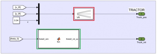
All data conversion necessary to make the simulation data usable in the VR sink is done in the 'Signal Shaping' sub-component. There are two type of movements driving this simulation model:

• Translations: This is the movement of bodies inside the model. Translations require a VR Signal Expander block (in red). This block expands input vectors into virtual world field vectors (which are required by the VR sink). Moreover, this block converts the x-y-z axis to x-z-y axis (The VR sink uses the y-axis as a vertical translation).
• Rotations: This is the rotation of bodies inside the model. The rotations require some shaping to be accepted into the VR file. The angles from the simulation model are first converted to a rotation matrix and, then, converted to an axis-angle rotation. This occurs inside the MATLAB Function blocks (in green). Furthermore, some differences in conventions are fixed inside these blocks (inverting rotations, correcting orientation differences).

Each area (inside 'Signal Shaping') contains an elaboration on the function of the shaping. For information on each signal, open the 'Signal Shaping' sub-component in the Simulink model.

VR Sink

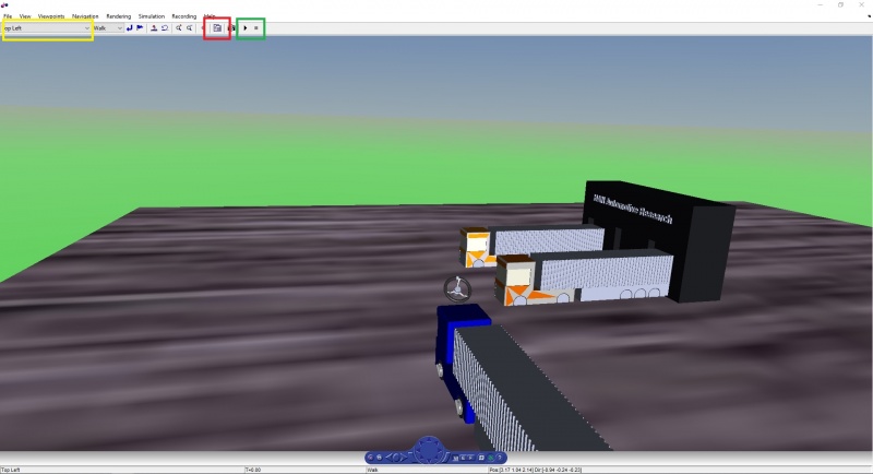
The 'SAV VR Sink' is the component to which all the signals are entered. Bodies can have a translation and/or a rotation. Double-click on the VR Sink to open the Virtual World Editor. This opens the window seen below.

• The yellow area is a view selector. Here, in the drop-down menu, several different views can be chosen to watch the animation from another viewpoint. Note: When a new view is selected, it takes some time before the view is shown.

• The red area contains the block parameters. These are the parameters for the VR Sink. Inside, for each object, the method of control can be selected (translation, rotation etc.). When a new box is checked, an input port is added to the VR Sink in the Simulink model. This is where the input can be connected. Note: If changes are made, first click the 'Apply' button, before 'OK' is clicked.

• The green area is the button to run the simulation. This will be done in a later phase of the tutorial.

VRealm Builder

Under File -> Open in Editor, the VR file is opened in VRealm Builder. This is where the virtual world is built and all objects are designed and placed. For more elaboration on building VR worlds, follow the V-Realm Builder Tutorial.

Running the Model

To run the simulation and animation model, the parameters must be loaded. To do this follow the steps below:

1. Open the file 'run_animation_SAV_semitrailer.m'. This file will open in the MATLAB command window.

2. Run this file. This should place several variables in the workspace of MATLAB.

3. Now open the Simulation model file 'SAV_anim_semi_trailer' (If not open already).

4. Open the 'animation' sub-component and double-click on the VR-Sink. This opens the animation viewer. Select view 'Top Left'.

5. Now the animation can be run. Press the 'play' button in Simulink of the Animation viewer. The vehicle will now perform the Autodocking manoeuvre.

6. During execution, an XY graph open. These are the coordinates of the semi-trailer rear-axle. This graph plots the position along with the execution of the animation.

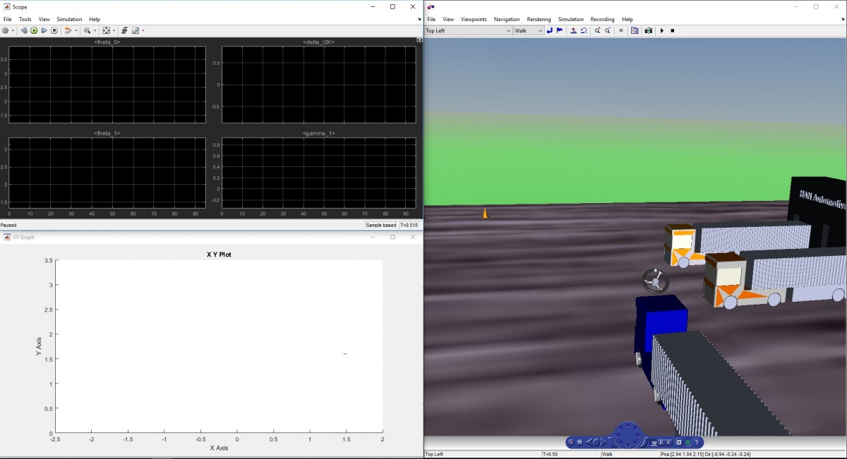
7. Now, the link between the simulation results and the animation will be made. Open the 'Signal Shaping' sub-component and select the scope. The results of the simulation are shown here. Create your own dashboard, with signals that you want to monitor, alongside the animation model. An example is seen below.

Here, the scope shows the following signals;

• theta_0: this is the yaw angle (orientation) of the tractor.
• theta_1: this is the yaw angle (orientation) of the trailer.
• delta_I2K: this is the steering angle of the wheels.
• gamma_1: this is the articulation angle between the trailer and the tractor.

Check if these signals are the same as the response seen in the animation. This clearly illustrates the link between the the simulation world and the results that can be expected in the real world.

Creating Plots

When a the simulation has been executed, the results can be seen in the Results Plot GUI.

1. Open the Results Plot GUI by double-clicking the block in the top-layer of the model.

2.